AI Academy

Predictive modeling plays a vital role in various industries, enabling organizations to make data-driven decisions. When it comes to modeling complex relationships, polynomial functions offer a powerful toolset. However, finding the optimal polynomial degree becomes a critical factor in striking the right balance between variance and bias. In this article, we explore the concepts of variance and bias in the context of polynomial functions and discuss their applications in real-world scenarios.

Understanding Variance and Bias:

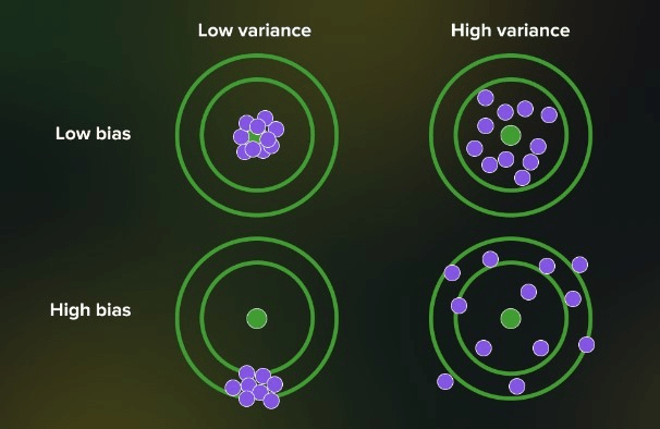
Variance and bias are two critical aspects of predictive modeling that impact a model’s accuracy and generalization capabilities. Bias represents the error caused by a model’s assumptions and simplifications, potentially leading to an oversimplified representation of the true relationship between input features and the target variable. High bias often results in underfitting, where the model fails to capture the underlying patterns and exhibits poor performance.

On the other hand, variance accounts for the sensitivity of a model to the training data. Models with high variance are overly complex, capturing noise and idiosyncrasies in the training set. This complexity often leads to overfitting, where the model performs exceptionally well on the training data but fails to generalize to unseen data.

Low-Degree Polynomial: High Bias, Low Variance:

In many real-world scenarios, low-degree polynomials, such as linear or quadratic functions, are valuable tools for predictive modeling. These polynomials offer a simple and interpretable representation of relationships between variables. They exhibit high bias, as they may not capture intricate patterns in the data. However, they often provide robust and stable predictions, as they are less sensitive to fluctuations in the training data. The applications of low-degree polynomials range from linear regression models predicting housing prices based on square footage and number of rooms to quadratic models used in financial forecasting.

High-Degree Polynomial: Low Bias, High Variance:

For complex relationships that low-degree polynomials struggle to capture, high-degree polynomials can be powerful tools. Cubic or higher-order polynomials provide a more flexible representation, allowing the model to fit the training data more closely. These models exhibit low bias and can accurately capture intricate patterns. However, they often suffer from high variance, leading to overfitting. Applications of high-degree polynomials include modeling the behavior of physical systems, analyzing population growth dynamics, or predicting stock market fluctuations based on historical data.

Striking the Right Balance:

Achieving the optimal balance between bias and variance is crucial for developing accurate and reliable models. Regularization techniques, such as L1 or L2 regularization, can be employed to control the complexity of high-degree polynomials, mitigating overfitting and reducing variance. These techniques add penalty terms to the model’s objective function, discouraging excessive complexity and helping achieve better generalization. Additionally, using validation techniques like cross-validation allows modelers to select the polynomial degree that maximizes performance on unseen data, striking the desired balance between bias and variance.

Applications and Considerations:

Choosing the right polynomial degree depends on the specific application and dataset. In fields like image processing, computer vision, and natural language processing, high-degree polynomials may be beneficial for capturing intricate patterns and achieving accurate predictions. However, it’s crucial to be mindful of the potential for overfitting and the need for extensive training data.

In contrast, low-degree polynomials find applications in areas such as economics, social sciences, and simple regression tasks. Their interpretability and stability make them suitable for scenarios where complex relationships are not prevalent.

Therefore, the choice of polynomial degree in predictive modeling determines the delicate balance between variance and bias. By understanding the trade-offs and leveraging regularization techniques, modelers can optimize model performance. Low-degree polynomials offer stability and interpretability at the cost of potential underfit.